# Deep Learning for Computer Vision ## an introduction **ISAE-SUPAERO, SDD, 18 Nov. 2025** Florient CHOUTEAU <!--v--> Slides : https://fchouteau.github.io/isae-intro-to-cnns Notebooks : https://github.com/SupaeroDataScience/deep-learning/tree/main/vision <!--v--> 6 hours hands-on session to discover deep learning for computer vision  <!-- .element: height="40%" width="40%" --> <!--v--> ### Who ? <img src="static/img/ads_logo.jpg" alt="" width="128px" height="128px" style="background:none; border:none; box-shadow:none;"/> - **Florient CHOUTEAU**, SDD 2015-2016 🎂 - eXpert in Artificial Intelligence for Space Systems at **Airbus Defence and Space** - Computer Vision Team (Earth Observation, Space Exploration, Space Domain Awareness) - Specialized in Satellite Imagery Processing & Deep Learning - Daily job revolving around Machine Learning + Satellite Imagery - Information extraction - **Image processing** - Research stuff Any question ? contact me on slack ! PS : I also have an internship open ;) <!--v--> # outcomes - how do we use neural networks when we have image ? - notions of convolutional neural networks for image classification - how we use CNNs to analyse and process (satellite) images - hands-on : perfect your torch / deep learning skills <!--v--> This is a "hands-on", not a full class **Resources on Deep Learning** - [The Little Book of Deep Learning](https://fleuret.org/francois/lbdl.html) **Resources on Deep Learning for Computer Vision** - [Stanford CS231n](http://cs231n.stanford.edu/schedule.html) - [M2 MVA](...) - [https://d2l.ai/index.html](https://d2l.ai/index.html) <!--s--> # Résumé de l'épisode précédent <!--v--> ### What you did last time - artificial neural networks (mlp) + backpropagation - first training loops in pytorch on fashion mnist "flattened" - discovered "callbacks" (early stopping), optimizers (sgd, adam), dropout <!--v--> > Artificial neural networks are computational graphs (architectures) that comprised of linear operations with parameters (neurons) and non-linear activation functions 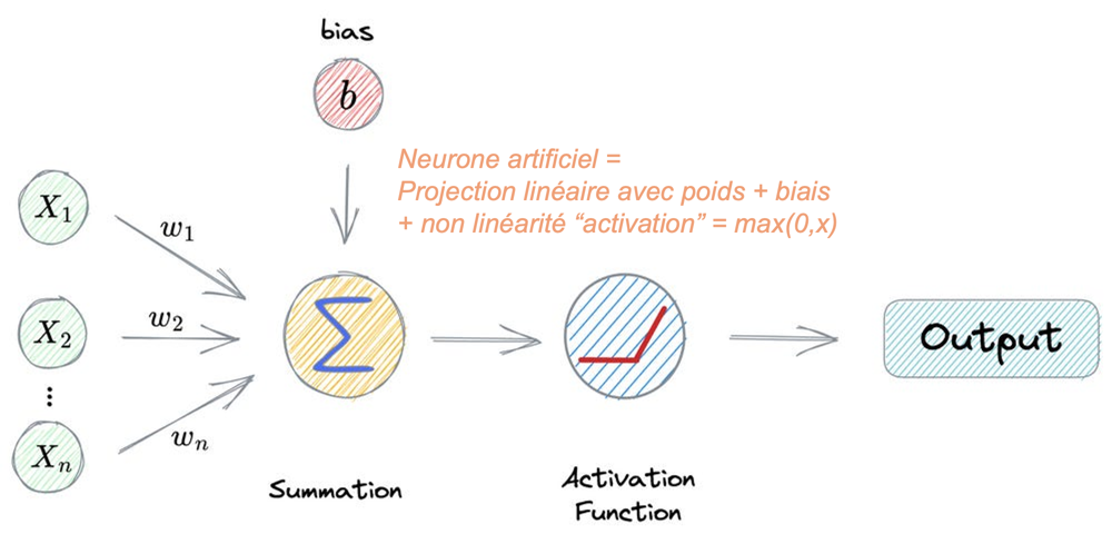 <!-- .element height="50%" width="50%" --> <!--v--> > The parameters (also called weights) of these neural networks can be learned with backpropagation. 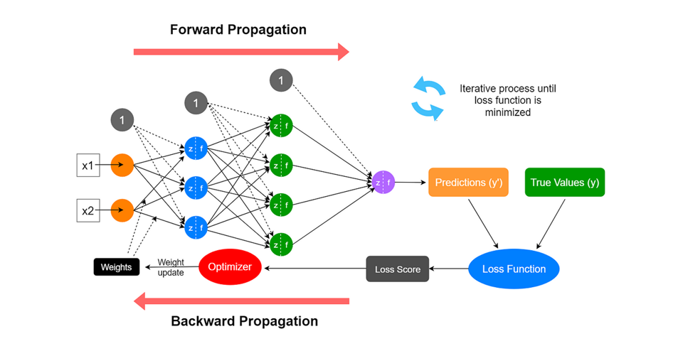 <!-- .element height="50%" width="50%" --> <!--v--> > Deep Learning is the art of training increasingly more complex (deeper) architectures end-to-end with increasingly more data. > > Deep Learning allows hierarchical learning of features adapted to the problem 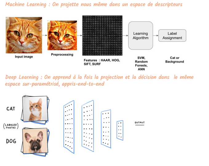 <!-- .element height="40%" width="40%" --> <!--v--> > Modern tools like pytorch allow you to write and train your architectures without worrying about low-level maths stuff.  <!-- .element height="50%" width="50%" --> <!--v--> Deep Learning is about scale : of data, of compute, of parameters  <!-- .element height="75%" width="75%" --> <!--v--> ### Deep Learning, with pytorch 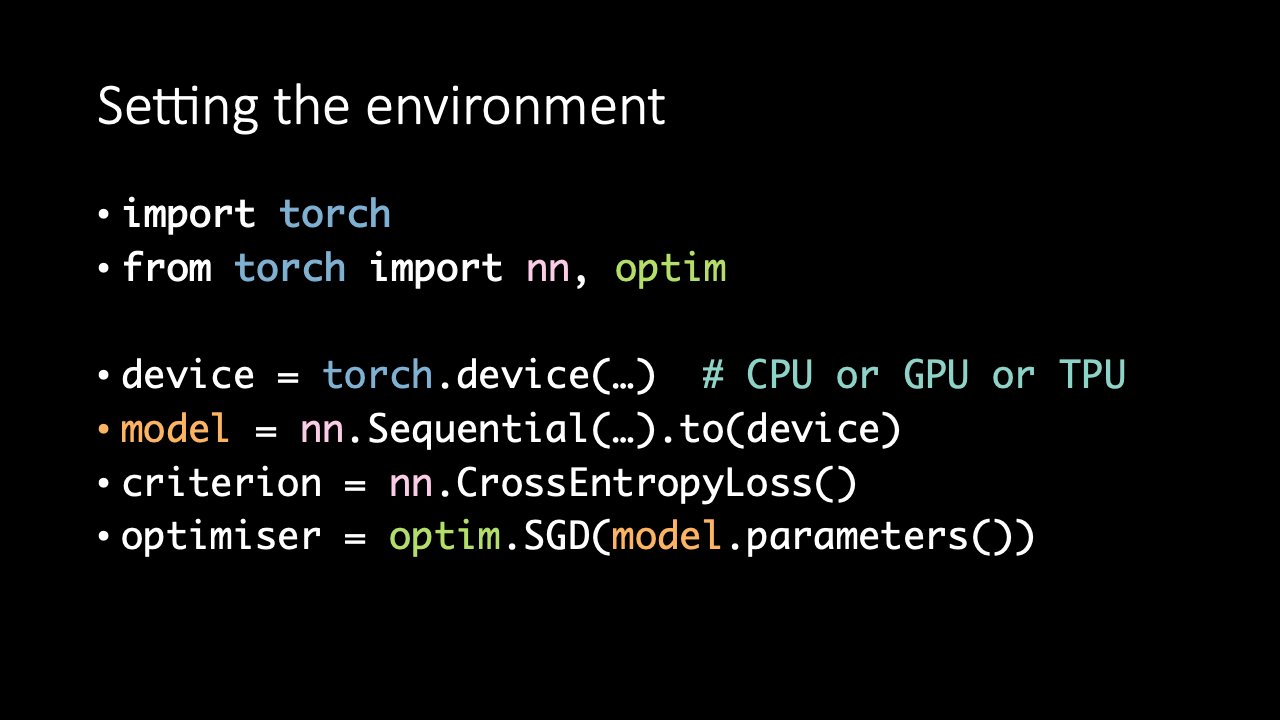 <!-- .element height="50%" width="50%" --> <!--v--> ### Deep Learning, with pytorch 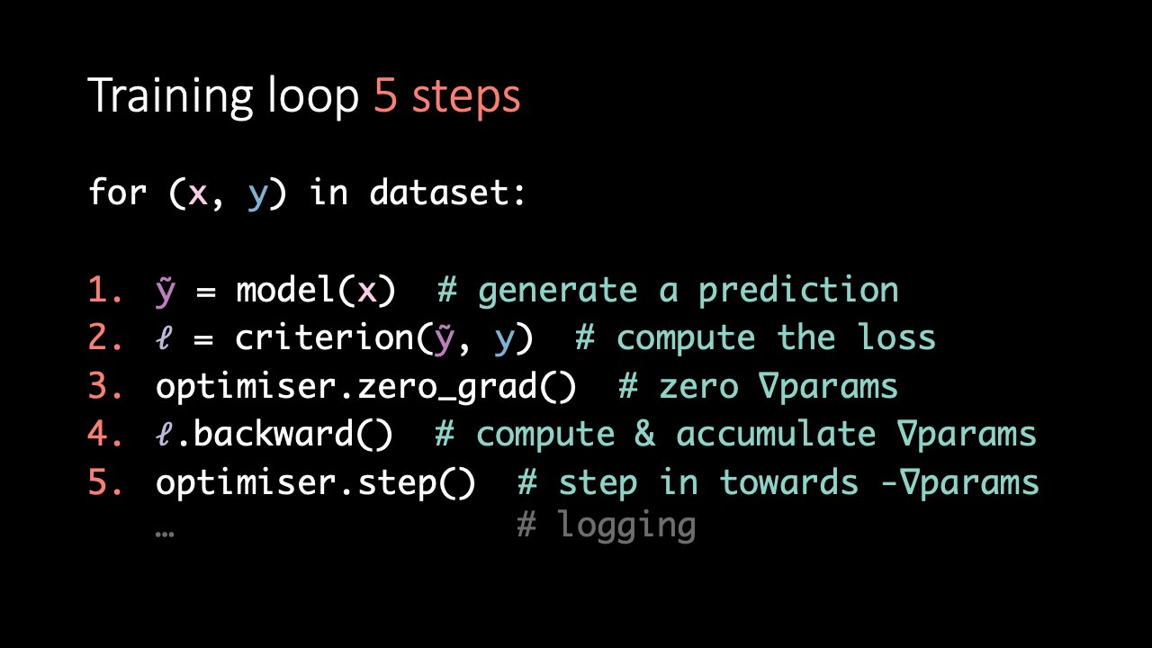 <!-- .element height="50%" width="50%" --> <!--s--> # Neural Networks # for Computer Vision <!--v--> **What to do when you have images ?** 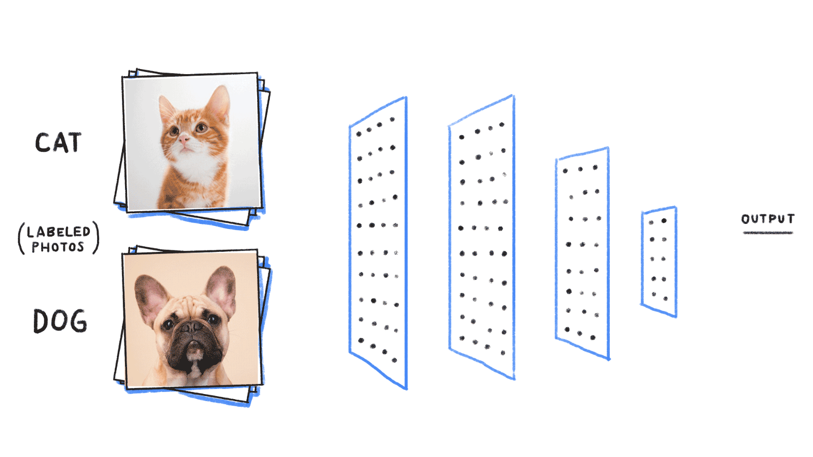 <!-- .element height="50%" width="50%" --> <!--v--> **This could work... but is it efficient ?** 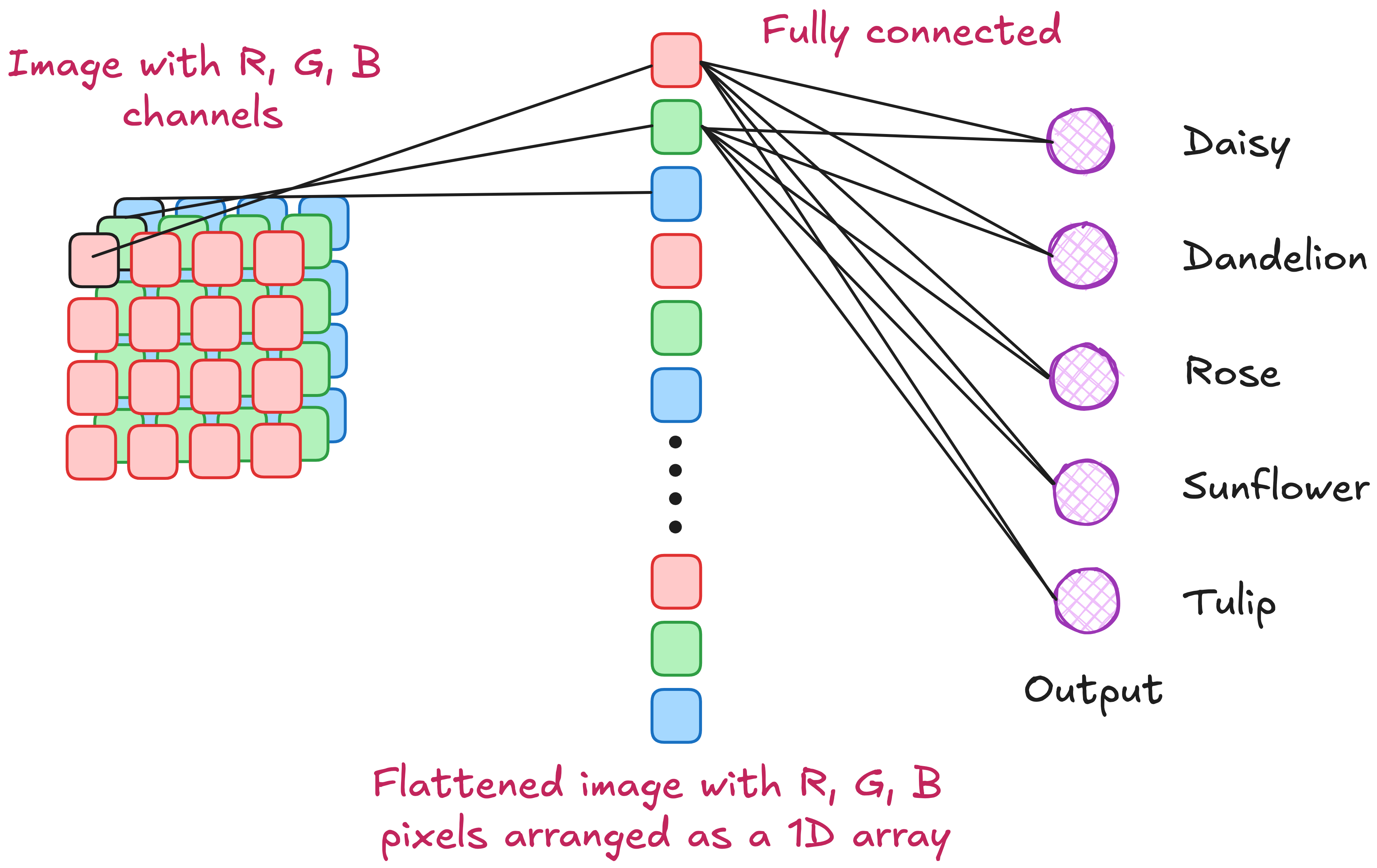 <!-- .element height="50%" width="50%" --> <!--v--> **Convolution (1D)**  <!-- .element height="40%" width="40%" --> <!--v--> **Kernel filtering (2D)** 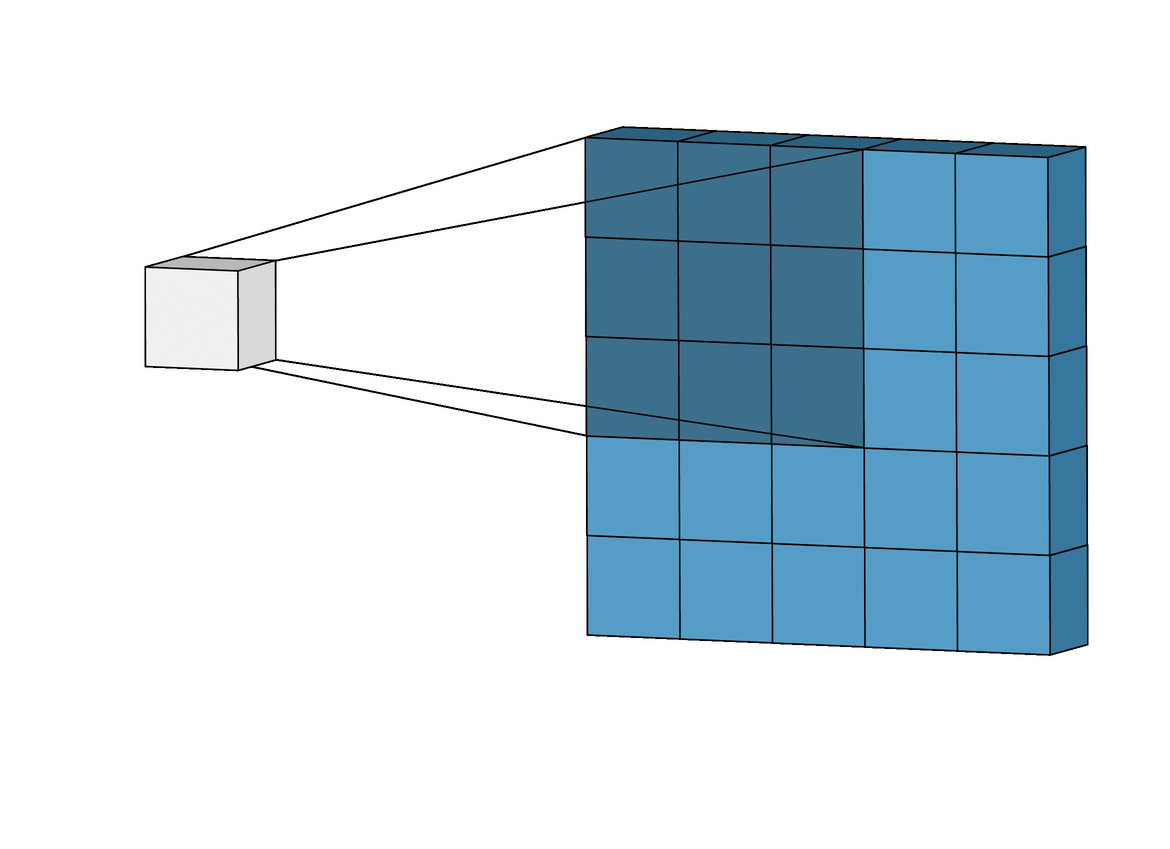 <!-- .element height="30%" width="30%" --> <!--v--> **Kernel filtering (2D)** 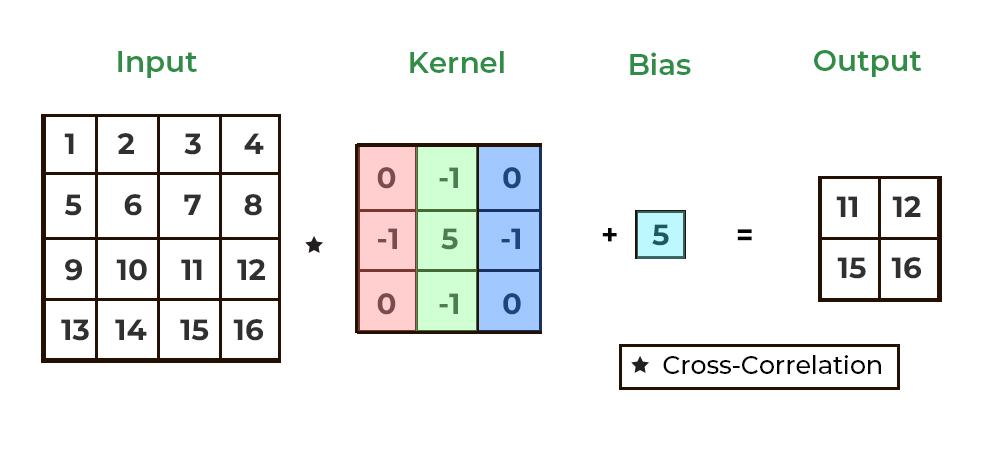 <!-- .element height="30%" width="30%" --> <!--v--> **You can hand-craft filters to reach certain effects** 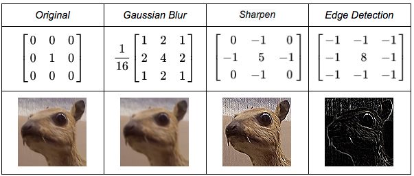 <!-- .element height="60%" width="60%" --> <!--v--> **What if we learned the filters ?** 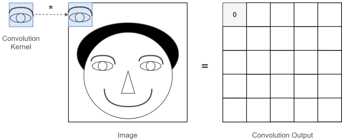 <!-- .element height="60%" width="40%" --> <!--v--> **from learnable MLPs to learnable convolutions** 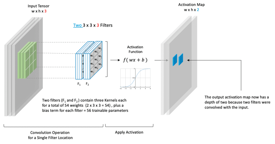 <!-- .element height="50%" width="50%" --> <!--v--> **from 2d convolutions to tensorial convolutions** 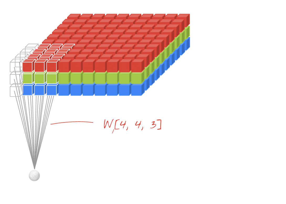 <!-- .element height="50%" width="50%" --> <!--v--> **Convolutional Neural Networks** 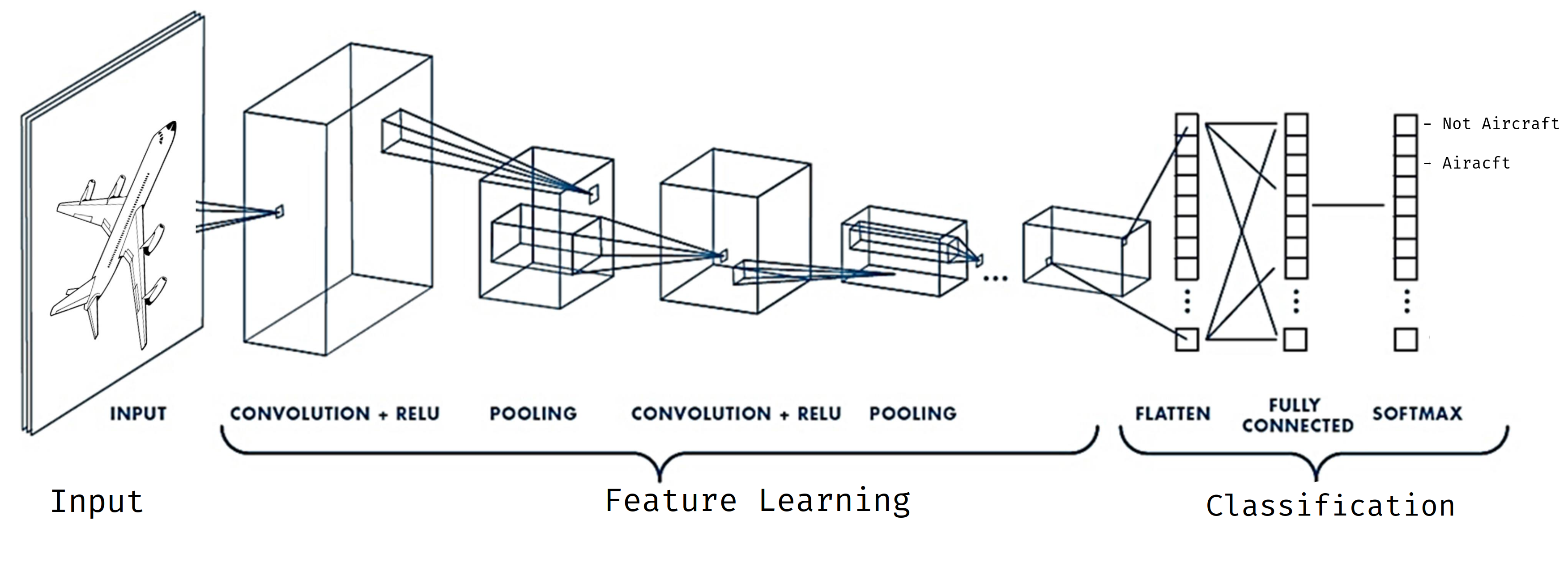 <!-- .element height="60%" width="60%" --> <!--v--> **Convolutions ?**  <!-- .element height="40%" width="40%" --> [useful link](https://github.com/vdumoulin/conv_arithmetic) <!--v--> **Pooling ?** 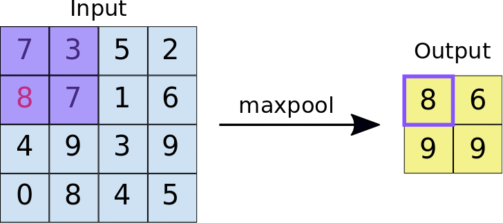 <!-- .element height="40%" width="40%" --> <!--v--> **nn.Linear ?** 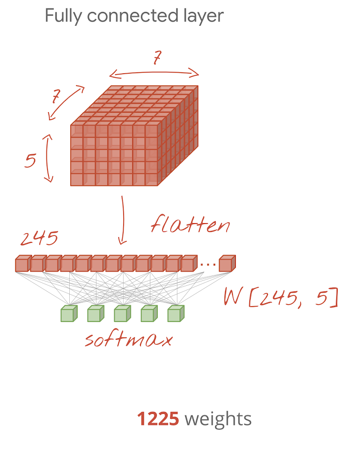 <!-- .element height="40%" width="40%" --> <!--v--> **Computing shape** 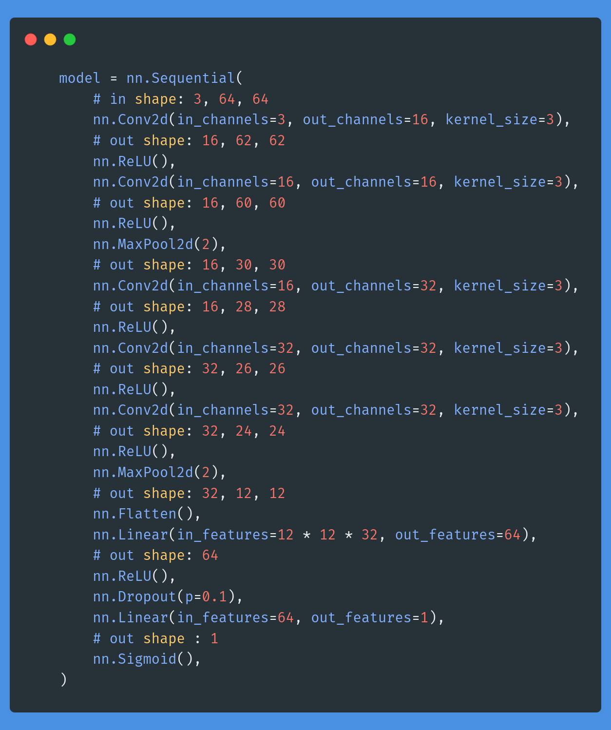 <!-- .element height="35%" width="35%" --> <!--v--> **ConvNets works because we assume inputs are images**  <!-- .element height="60%" width="60%" --> <!--v--> **ConvNets "solved" image classification**  <!-- .element height="60%" width="60%" --> <!--s--> ## CNN architectures & Transfer Learning <!--v--> How do I know the number of filters, conv etc for my use case ? <!--v--> [VGG16, 2014](https://arxiv.org/abs/1409.1556)  <!-- .element height="60%" width="60%" --> <!--v--> [Residual Networks (ResNets), 2015](https://arxiv.org/abs/1512.03385) 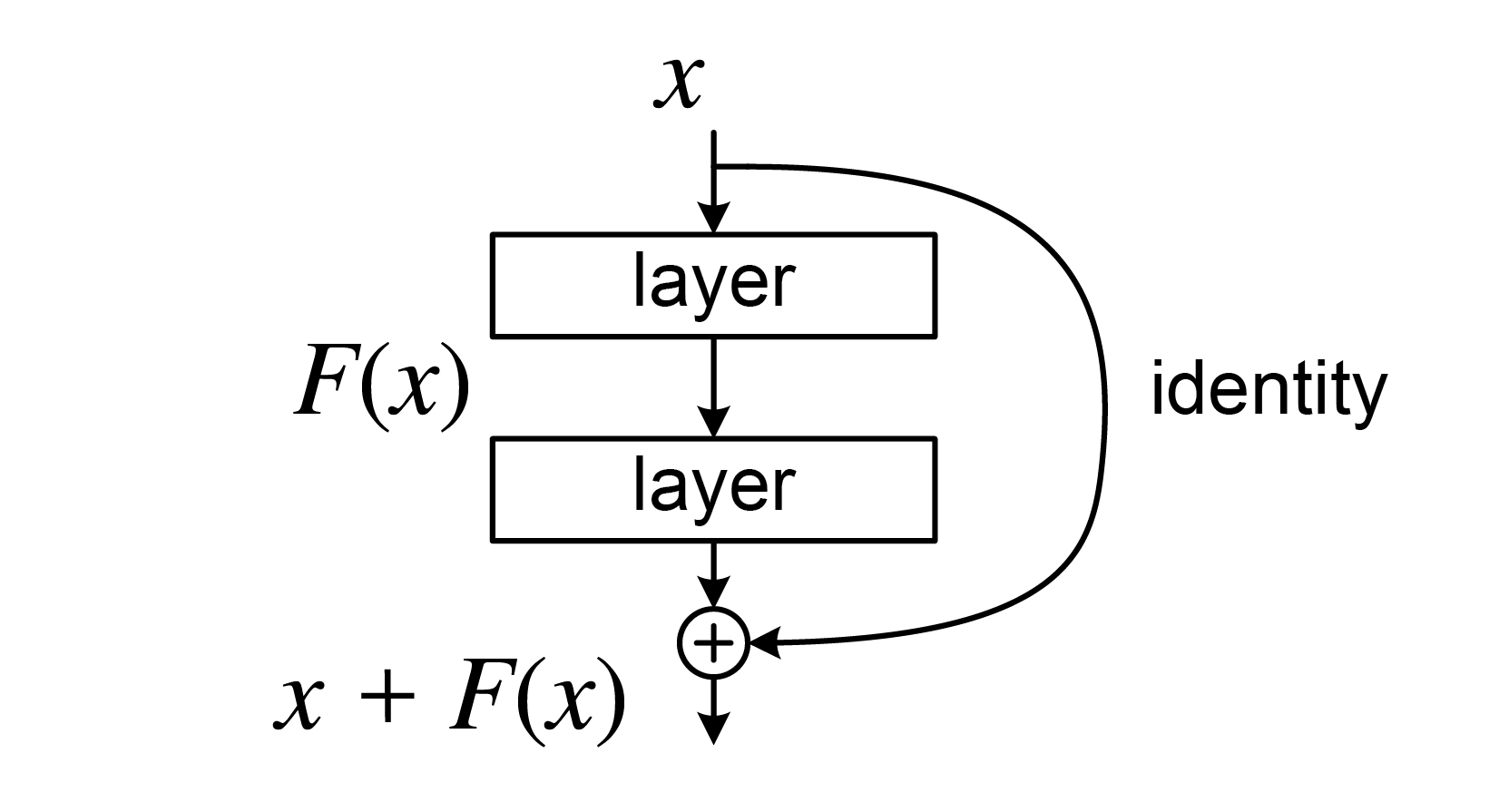 <!-- .element height="60%" width="60%" --> <!--v--> 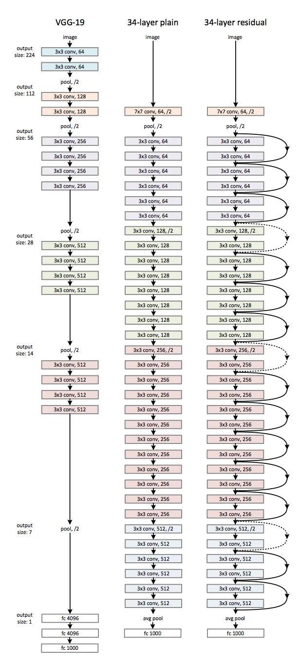 <!-- .element height="50%" width="25%" --> <!--v--> 🤯 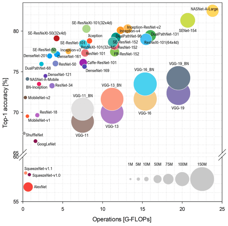 [Well written paper :ConvNext, a ConvNet for the 2020s](https://arxiv.org/abs/2201.03545) <!--v--> In practice  <!-- .element height="35%" width="35%" --> ```text ResNet( (conv1): Conv2d(3, 64, kernel_size=(7, 7), stride=(2, 2), padding=(3, 3), bias=False) (bn1): BatchNorm2d(64, eps=1e-05, momentum=0.1, affine=True, track_running_stats=True) (relu): ReLU(inplace=True) (maxpool): MaxPool2d(kernel_size=3, stride=2, padding=1, dilation=1, ceil_mode=False) (layer1): Sequential( (0): BasicBlock( (conv1): Conv2d(64, 64, kernel_size=(3, 3), stride=(1, 1), padding=(1, 1), bias=False) (bn1): BatchNorm2d(64, eps=1e-05, momentum=0.1, affine=True, track_running_stats=True) (relu): ReLU(inplace=True) (conv2): Conv2d(64, 64, kernel_size=(3, 3), stride=(1, 1), padding=(1, 1), bias=False) (bn2): BatchNorm2d(64, eps=1e-05, momentum=0.1, affine=True, track_running_stats=True) ) (1): BasicBlock( (conv1): Conv2d(64, 64, kernel_size=(3, 3), stride=(1, 1), padding=(1, 1), bias=False) (bn1): BatchNorm2d(64, eps=1e-05, momentum=0.1, affine=True, track_running_stats=True) (relu): ReLU(inplace=True) (conv2): Conv2d(64, 64, kernel_size=(3, 3), stride=(1, 1), padding=(1, 1), bias=False) (bn2): BatchNorm2d(64, eps=1e-05, momentum=0.1, affine=True, track_running_stats=True) ) ) (layer2): Sequential( (0): BasicBlock( (conv1): Conv2d(64, 128, kernel_size=(3, 3), stride=(2, 2), padding=(1, 1), bias=False) (bn1): BatchNorm2d(128, eps=1e-05, momentum=0.1, affine=True, track_running_stats=True) (relu): ReLU(inplace=True) (conv2): Conv2d(128, 128, kernel_size=(3, 3), stride=(1, 1), padding=(1, 1), bias=False) (bn2): BatchNorm2d(128, eps=1e-05, momentum=0.1, affine=True, track_running_stats=True) (downsample): Sequential( (0): Conv2d(64, 128, kernel_size=(1, 1), stride=(2, 2), bias=False) (1): BatchNorm2d(128, eps=1e-05, momentum=0.1, affine=True, track_running_stats=True) ) ) (1): BasicBlock( (conv1): Conv2d(128, 128, kernel_size=(3, 3), stride=(1, 1), padding=(1, 1), bias=False) (bn1): BatchNorm2d(128, eps=1e-05, momentum=0.1, affine=True, track_running_stats=True) (relu): ReLU(inplace=True) (conv2): Conv2d(128, 128, kernel_size=(3, 3), stride=(1, 1), padding=(1, 1), bias=False) (bn2): BatchNorm2d(128, eps=1e-05, momentum=0.1, affine=True, track_running_stats=True) ) ) (layer3): Sequential( (0): BasicBlock( (conv1): Conv2d(128, 256, kernel_size=(3, 3), stride=(2, 2), padding=(1, 1), bias=False) (bn1): BatchNorm2d(256, eps=1e-05, momentum=0.1, affine=True, track_running_stats=True) (relu): ReLU(inplace=True) (conv2): Conv2d(256, 256, kernel_size=(3, 3), stride=(1, 1), padding=(1, 1), bias=False) (bn2): BatchNorm2d(256, eps=1e-05, momentum=0.1, affine=True, track_running_stats=True) (downsample): Sequential( (0): Conv2d(128, 256, kernel_size=(1, 1), stride=(2, 2), bias=False) (1): BatchNorm2d(256, eps=1e-05, momentum=0.1, affine=True, track_running_stats=True) ) ) (1): BasicBlock( (conv1): Conv2d(256, 256, kernel_size=(3, 3), stride=(1, 1), padding=(1, 1), bias=False) (bn1): BatchNorm2d(256, eps=1e-05, momentum=0.1, affine=True, track_running_stats=True) (relu): ReLU(inplace=True) (conv2): Conv2d(256, 256, kernel_size=(3, 3), stride=(1, 1), padding=(1, 1), bias=False) (bn2): BatchNorm2d(256, eps=1e-05, momentum=0.1, affine=True, track_running_stats=True) ) ) (layer4): Sequential( (0): BasicBlock( (conv1): Conv2d(256, 512, kernel_size=(3, 3), stride=(2, 2), padding=(1, 1), bias=False) (bn1): BatchNorm2d(512, eps=1e-05, momentum=0.1, affine=True, track_running_stats=True) (relu): ReLU(inplace=True) (conv2): Conv2d(512, 512, kernel_size=(3, 3), stride=(1, 1), padding=(1, 1), bias=False) (bn2): BatchNorm2d(512, eps=1e-05, momentum=0.1, affine=True, track_running_stats=True) (downsample): Sequential( (0): Conv2d(256, 512, kernel_size=(1, 1), stride=(2, 2), bias=False) (1): BatchNorm2d(512, eps=1e-05, momentum=0.1, affine=True, track_running_stats=True) ) ) (1): BasicBlock( (conv1): Conv2d(512, 512, kernel_size=(3, 3), stride=(1, 1), padding=(1, 1), bias=False) (bn1): BatchNorm2d(512, eps=1e-05, momentum=0.1, affine=True, track_running_stats=True) (relu): ReLU(inplace=True) (conv2): Conv2d(512, 512, kernel_size=(3, 3), stride=(1, 1), padding=(1, 1), bias=False) (bn2): BatchNorm2d(512, eps=1e-05, momentum=0.1, affine=True, track_running_stats=True) ) ) (avgpool): AdaptiveAvgPool2d(output_size=(1, 1)) (fc): Linear(in_features=512, out_features=2, bias=True) ) ``` <!--v--> Introducing [timm](https://github.com/huggingface/pytorch-image-models) 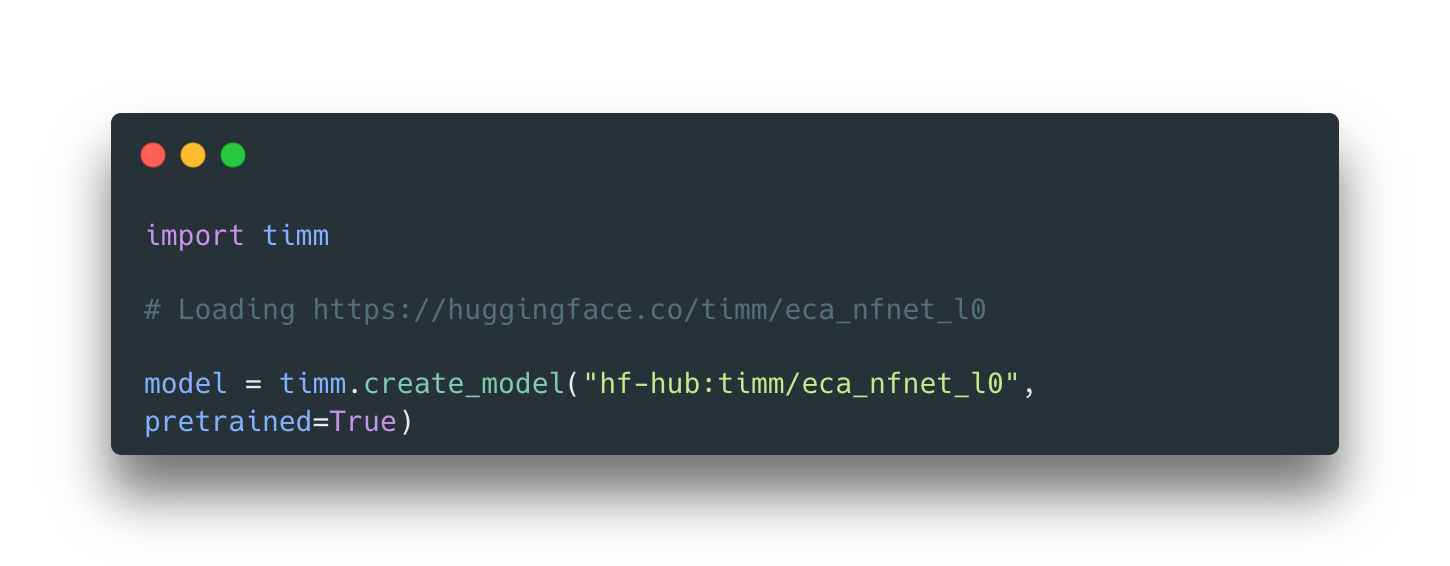 <!-- .element height="60%" width="60%" --> <!--v--> Transfer Learning 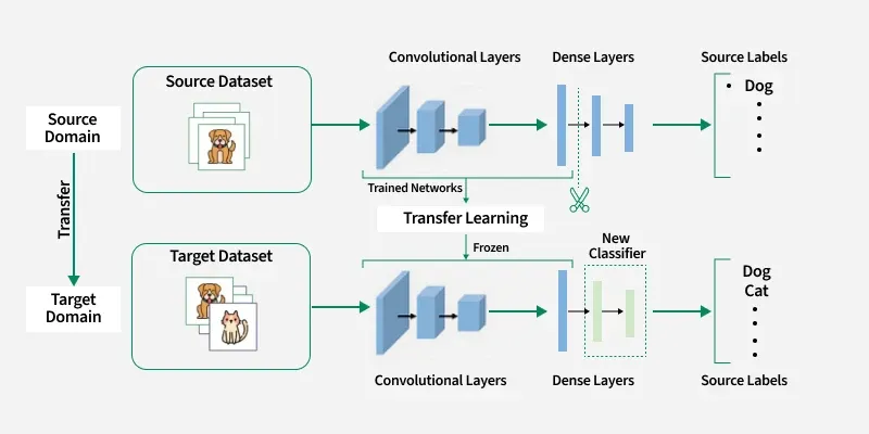 <!-- .element height="60%" width="60%" --> <!--v--> Finetuning 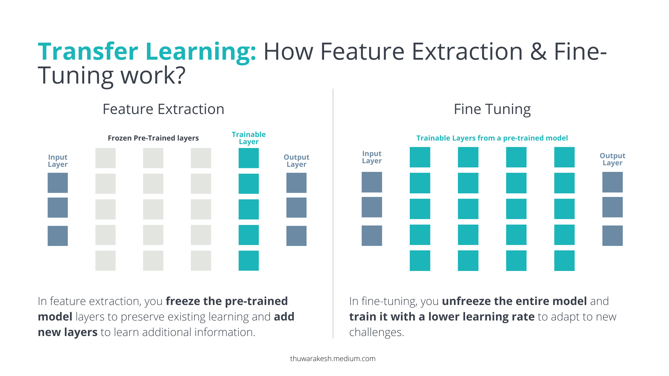 <!-- .element height="60%" width="60%" --> - Transfer learning : We take the features as is, and freeze the "encoder's" layers - Finetuning : Usually we don't freeze all weights <!--v--> ### References - [Understand Convolutional Neural Networks](https://learnopencv.com/understanding-convolutional-neural-networks-cnn/) - [Convolution Arithmetics](hub.com/vdumoulin/conv_arithmetic?tab=readme-ov-file) <!--s--> # Hands-on 1 : CNNs and Classification <!--v--> ### Objectives - Launch notebooks on Colab - Build an intuition over convolutions and CNNs - Train a basic CNN on a small training set - Plot the metrics & ROC curve on a small test set - Discover the world of hyperparameter tuning <!--v--> ### Outcomes - Build an intuition over convolutions and CNNs for image processing - Handle a dataset of images, do some basic data exploration - Train & evaluate your first CNN on a simple dataset - Go beyound accuracy to diagnose your model <!--v--> ### Context: Earth Observation 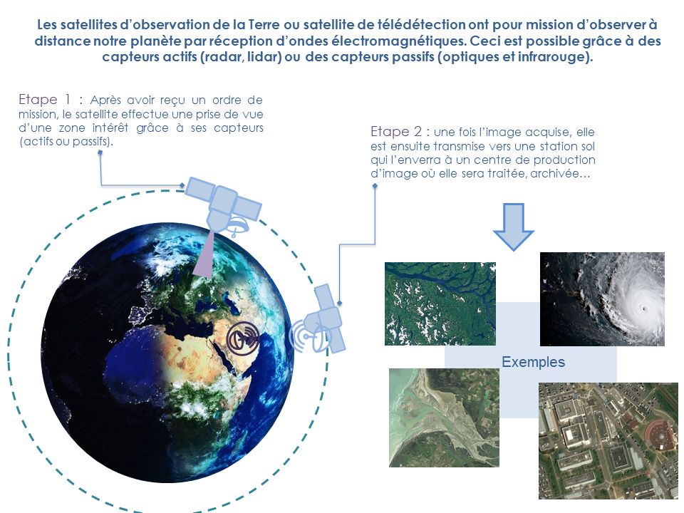 <!-- .element: width="60%" height="60%"--> <!--v--> ### Context: DL on Satellite Imagery A lot of use cases : - Land Use / Land Cover cartography - Urban Cartography (building, roads, damage assessment...) - Various objects detections (ships, vehicles...)  <!-- .element: width="60%" height="60%"--> <!--v--> ### Context: DL on Satellite Imagery Can also be used for "image processing" : - Denoising - Super Resolution 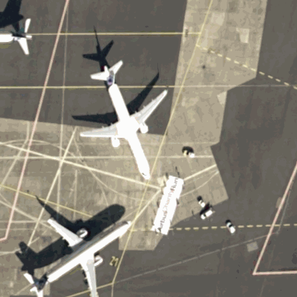 <!-- .element: width="20%" height="20%"--> <!--v--> ### Context: Needles in haystacks 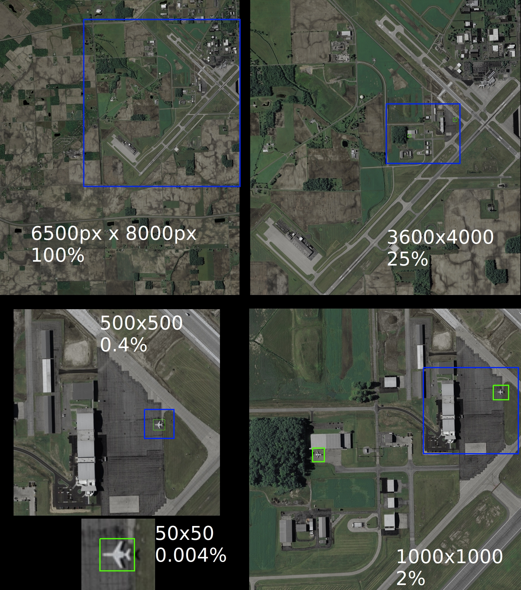 <!-- .element: width="40%" height="40%"--> <!--v--> ### Context: Cloud Detection 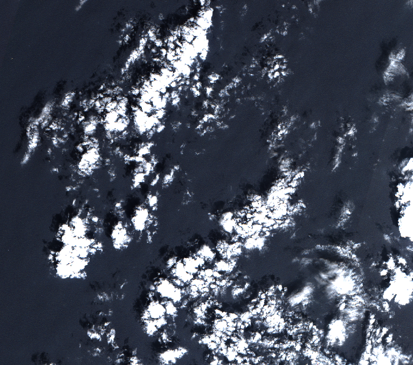 <!-- .element: width="40%" height="40%"--> <!--v--> ### Context: Cloud Detection 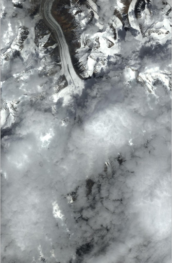 <!-- .element: width="25%" height="20%"--> <!--v--> ### Dataset description - 12800 train images (6400 cloudy, 6400 clear), size 64x64 - 640 test images (320 cloudy, 320 clear), size 64x64 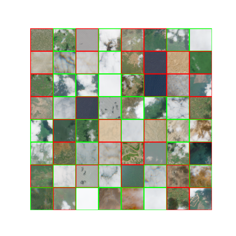 <!-- .element height="40%" width="40%" --> <!--v--> ### Dataset description - 64 big test images (256x256) 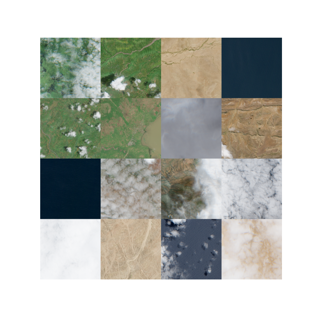 <!-- .element height="40%" width="40%" --> <!--v--> ### Let's go ! - 0_cnns.ipynb : You will get a grasp in image, convolutions and CNNs - 1_hands_on.ipynb : Train our first cloud detector using CNNs - 2_sliding_window.ipynnb : How to apply our detector to a big satellite image ? <!--v--> ### Let's go ! 1. Go to google colab 2. Import the first notebook & follow the guidelines 3. ... 4. Profit ! 5. If you're done... go to the next notebook ! <!--v--> ### Colab Guide <video data-autoplay controls width="720"> <source src="https://storage.googleapis.com/fchouteau-isae-deep-learning/static/colab_guide_proper.mp4" type="video/mp4"> </video> <!--v--> ### GPU ??? 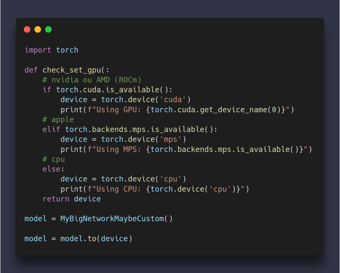 <!-- .element height="50%" width="50%" --> <!--v--> ### GPU ???  <!-- .element height="50%" width="50%" --> <!--v--> ### GPU ??? [Tutorial](http://d2l.ai/chapter_appendix-tools-for-deep-learning/colab.html) <!--s--> ## Extra : From CNN to Transformers <!--v--> 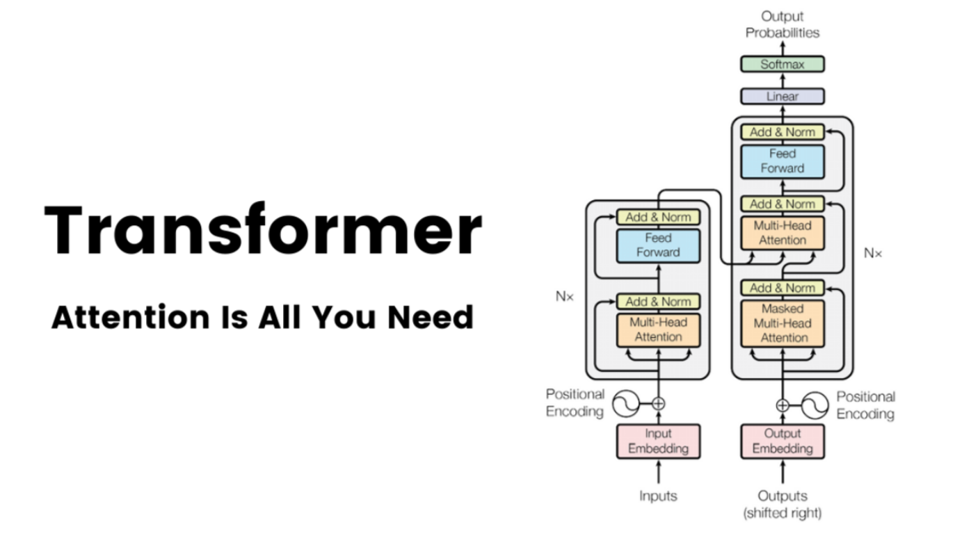 <!-- .element height="50%" width="50%" --> <!--v--> 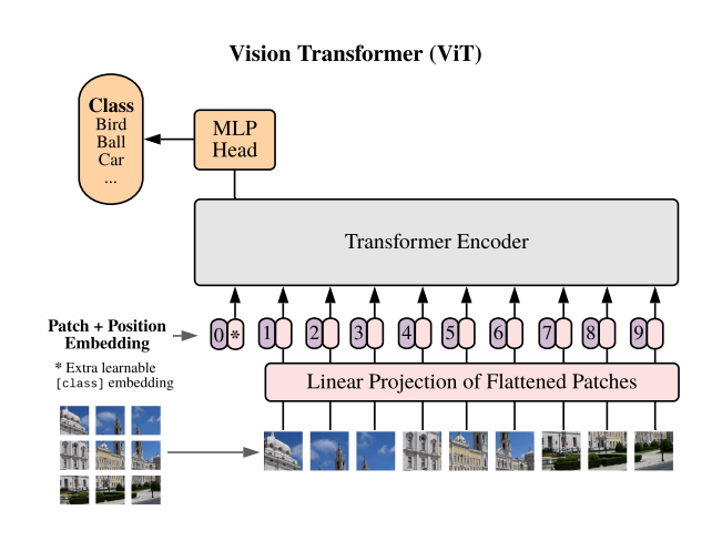 <!-- .element height="50%" width="50%" --> [An Image is Worth 16x16 Words](https://arxiv.org/abs/2010.11929) <!--v--> 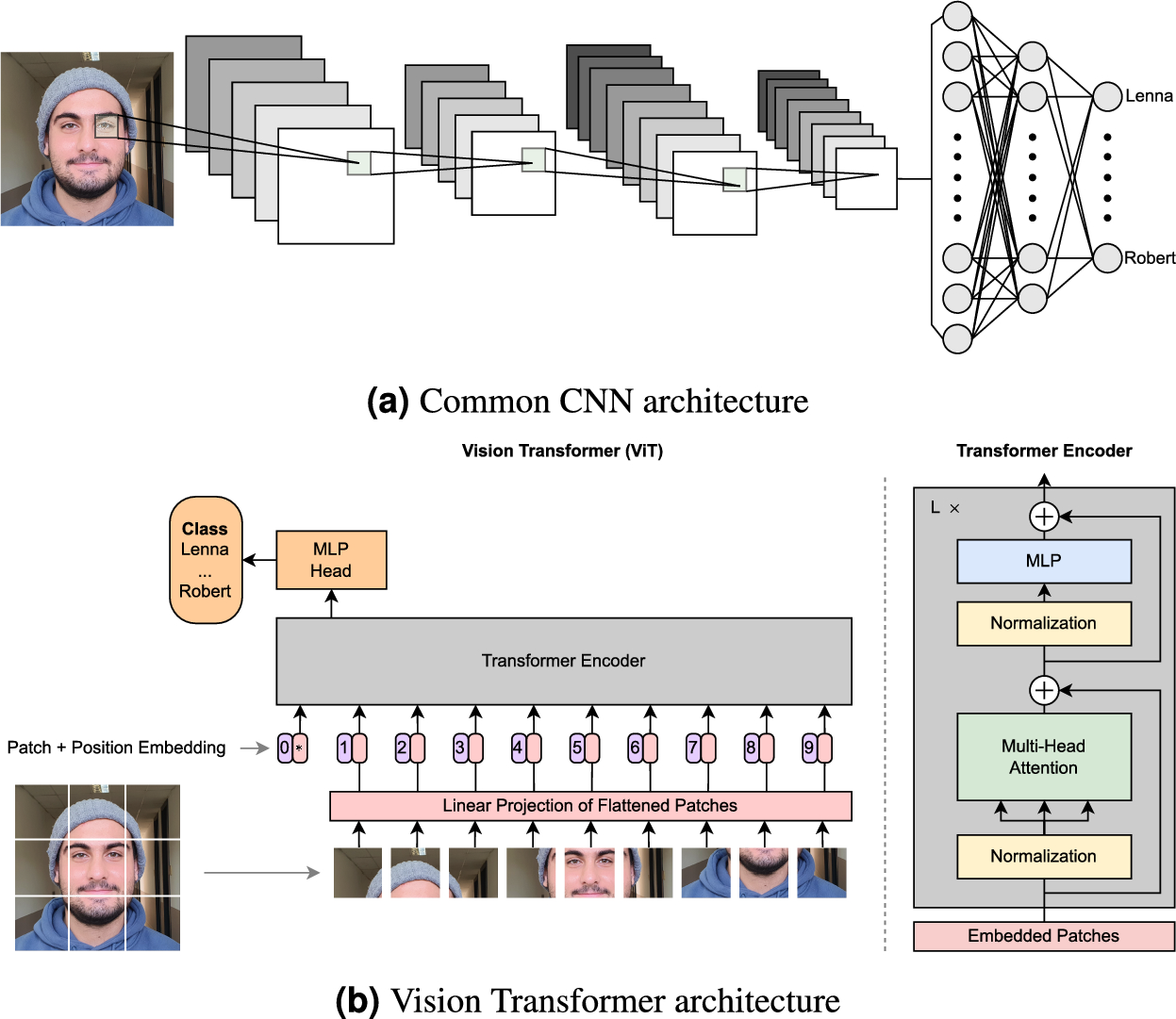 <!-- .element: style="width: 60%; height: 40%"--> <!--v--> RIP inductive biases 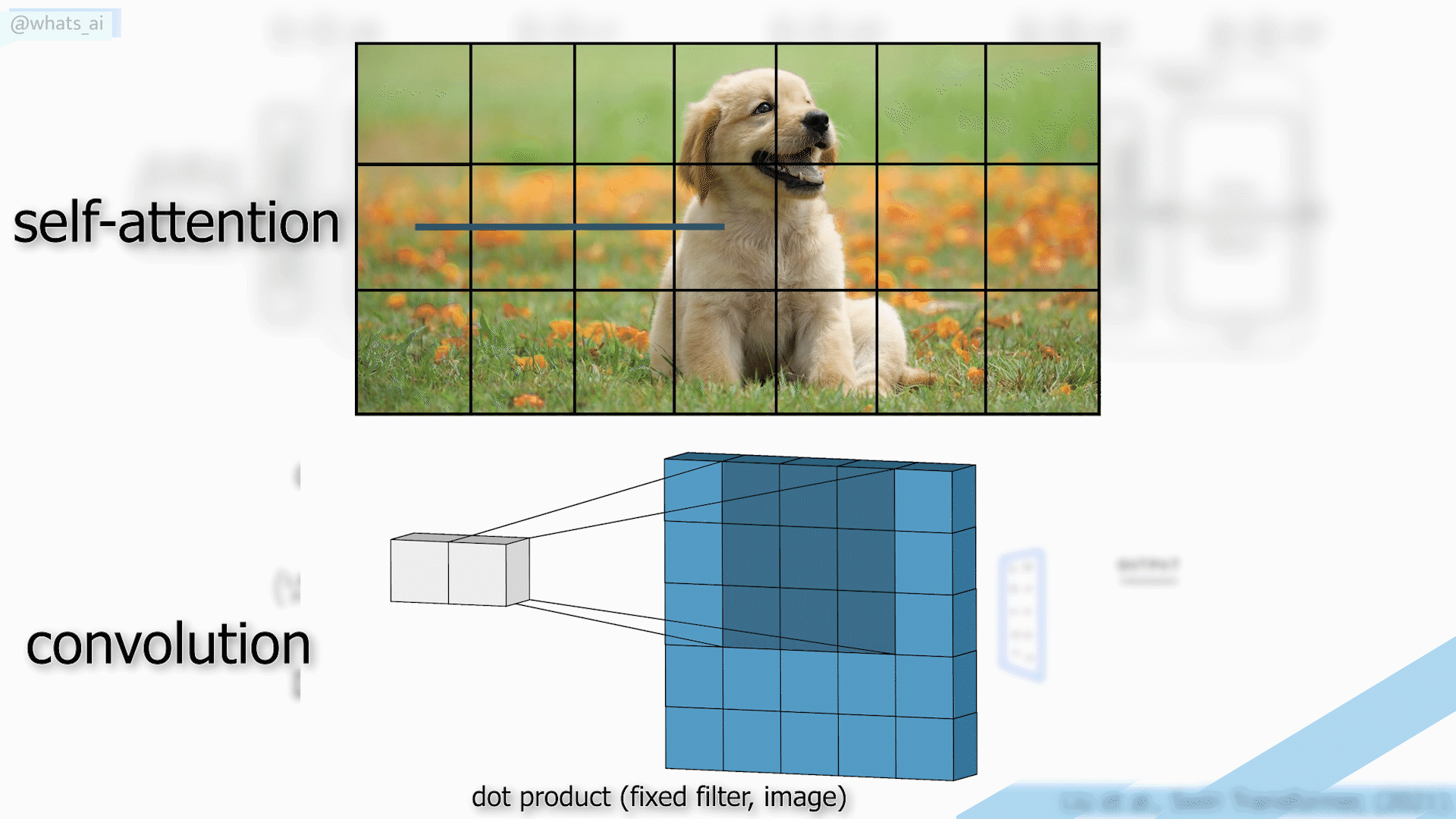 <!--v--> Links https://lbourdois.github.io/blog/nlp/Transformer/ https://nlp.seas.harvard.edu/annotated-transformer/ https://cs231n.stanford.edu/slides/2024/lecture_8.pdf <!--v--> [example use case](https://www.picsellia.com/post/are-transformers-replacing-cnns-in-object-detection) <!--s--> ## Extra ## Diagnosing Classifier performance <!--v--> ### Binary classification metrics 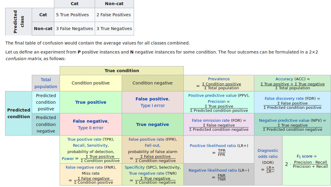 <!--v--> ### The ROC Curve 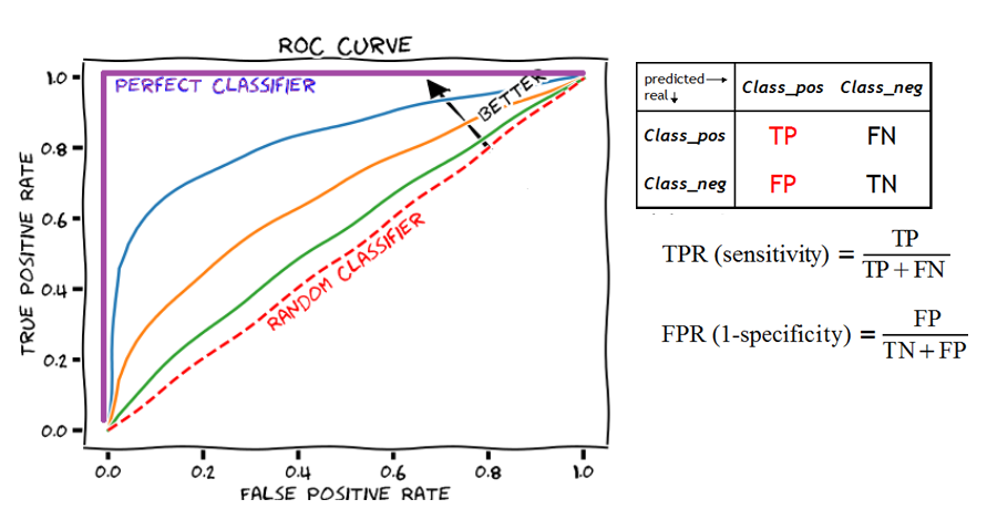 <!--v--> ### The ROC curve (visualized) 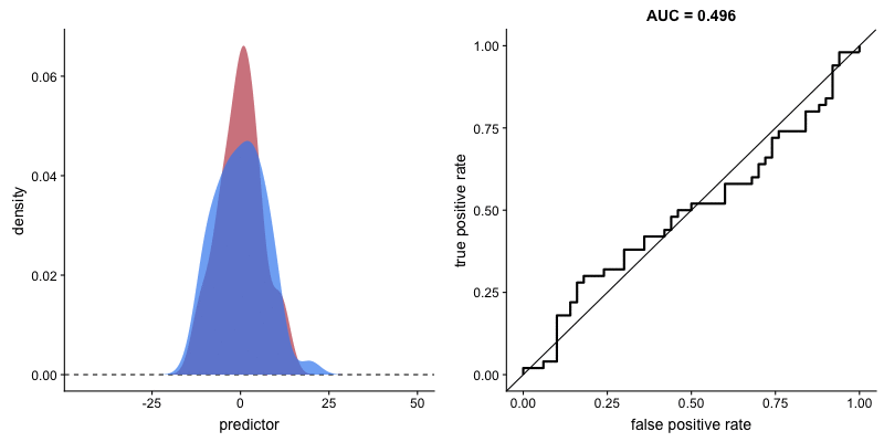 The shape of an ROC curve changes when a model changes the way it classifies the two outcomes. <!--v--> ### How to compute a ROC curve ? 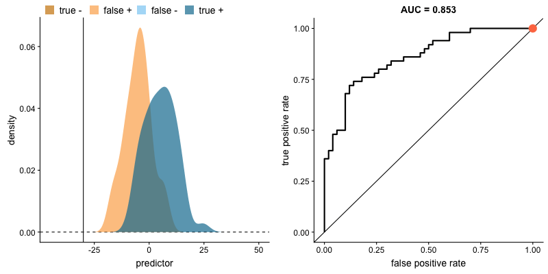 <!-- .element height="40%" width="40%" --> - y_pred = a list of probas, y_true = a list of 0 or 1 - vertical line : threshold value - red dot : FPR and TPR for the threshold - the curve is plotted for all available thresholds <!--v--> ### Precision & Recall Usually the most important things in imbalanced classification 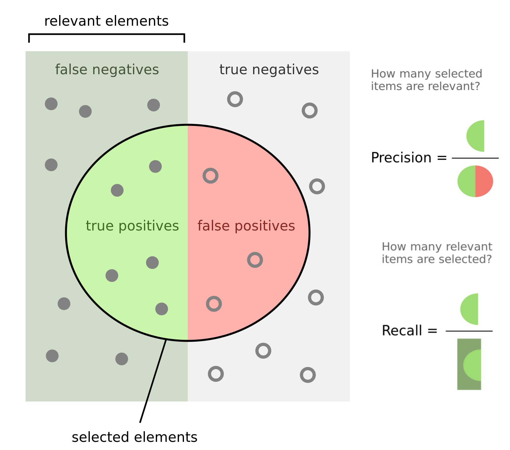 <!-- .element height="40%" width="40%" --> <!--v--> ### PR synthetic metric 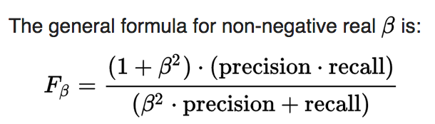 <!-- .element height="35%" width="35%" --> - beta = 1 => Recall & Precision weighted equally - beta > 1 => Emphasizes recall (not missing positive examples) - beta < 1 => Emphasizes precision (not doing ) <!--v--> ### The PR Curve 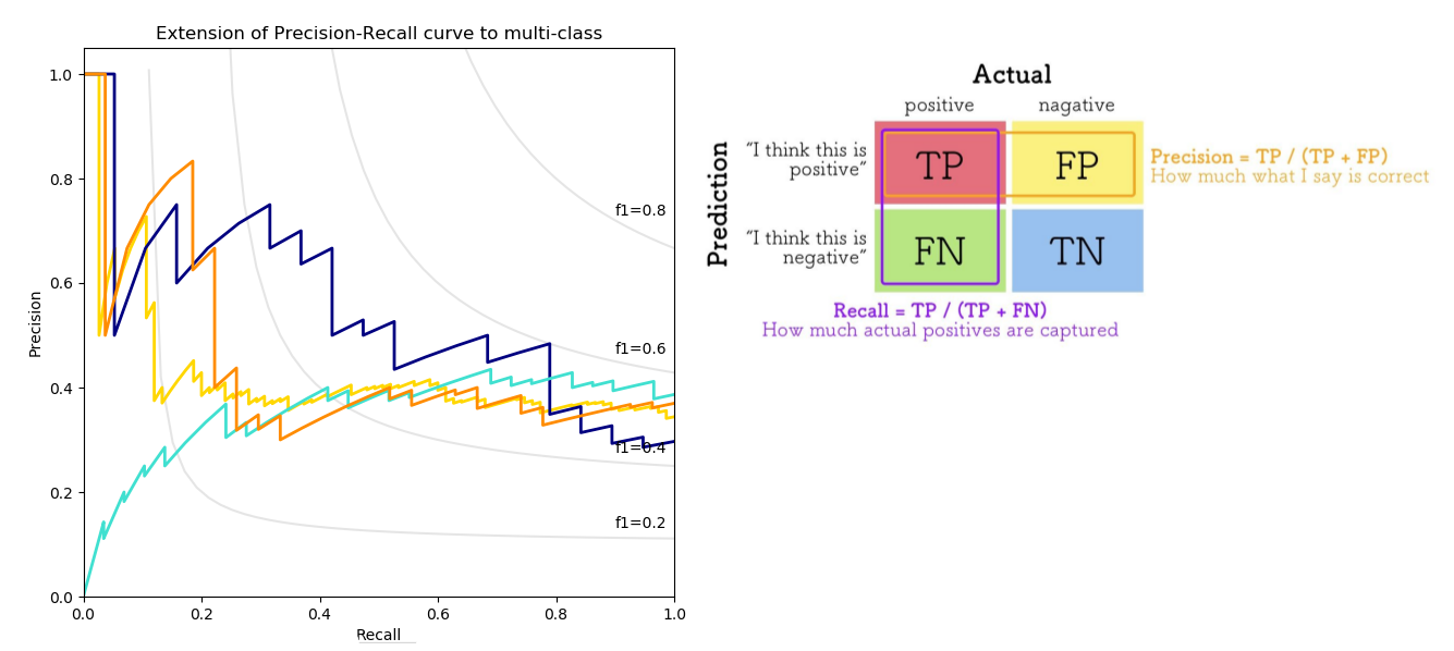 <!-- .element height="75%" width="75%" --> <!--v--> ### The PR Curve (visualized) 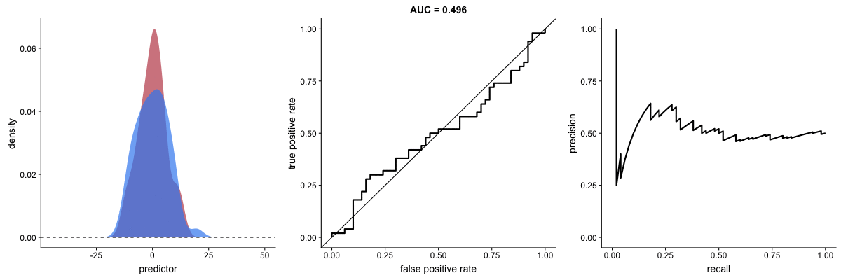 The shape of the precision-recall curve also changes when a model changes the way it classifies the two outcomes. <!--v--> ### Precision-Recall or ROC ? - Both curve can be used to select your trade-off - Precision-recall curve is more sensitive to class imbalance than an ROC curve - Example: Try computing your FPR on very imbalanced dataset 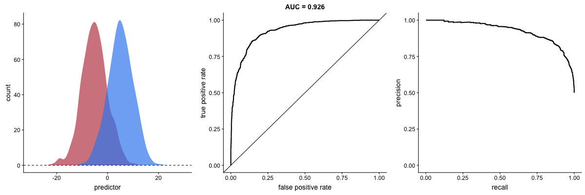 <!-- .element height="50%" width="50%" --> <!--v--> ### Curves Usage: Selecting trade-off 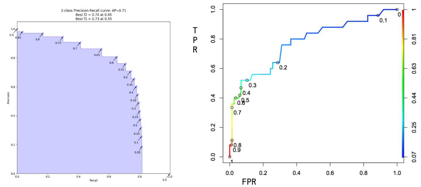 <!-- .element height="70%" width="70%" --> <!--v--> Readings: - https://lukeoakdenrayner.wordpress.com/2018/01/07/the-philosophical-argument-for-using-roc-curves/ - https://towardsdatascience.com/on-roc-and-precision-recall-curves-c23e9b63820c <!--s--> ## Extra : Pytorch Ecosystem <!--v--> ### high-level frameworks over pytorch - pytorch: define your models, autodifferenciation, **but you write the rest** - hl library: training loops, callbacks, distribution etc... 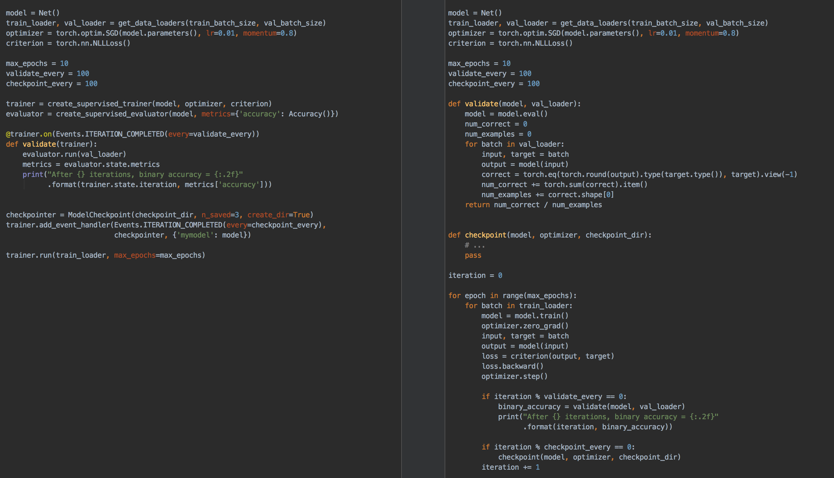 <!-- .element height="50%" width="50%" --> <!--v--> ### high-level frameworks over pytorch 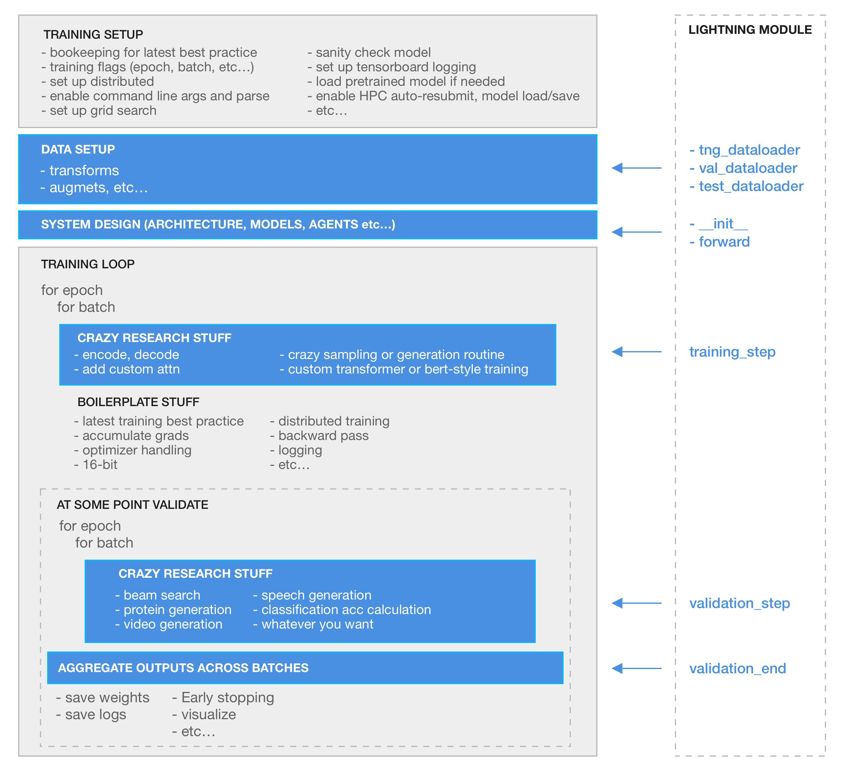 <!-- .element height="40%" width="40%" --> <!--v--> ###  <!-- .element: width="15%" height="15%"--> - [pytorch-ignite](https://github.com/skorch-dev/skorch) : a high-level deep learning library based on top of pytorch - Reduce boilerplate code (training loops, early stopping, logging...) - Extensible, based on experiment management <!--v--> ### Pytorch Ecosystem - There are other high-level frameworks based on pytorch: [Skorch](https://github.com/skorch-dev/skorch), [Lightning](https://github.com/williamFalcon/pytorch-lightning). - All of them have their pros and cons - [There is a huge ecosystem based around pytorch](https://pytorch.org/ecosystem/)  <!-- .element: style="width: 25%; height: 25%"-->
